Fishery Areas Closed Due to Oil Present: 05/25/10

This is my Google Earth image of my FisheryClosing.KZM file. I worked on this for over ten hours, running into problemson just about every step. Then on my last attempt it worked perfectly. I don't exactly know what I was doing wrong. But I sure am glad to be through.

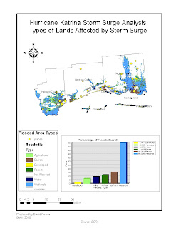
Hurricane Katrina:Types of Lands Affected by Storm Surge

I have included the approximate areas which flooded during Hurricane Katrina. I have indicated the land types that flooded includ Agricultural,Barren,Developed,Forest,Not
Flooded,Water, and Wetlands. The chart also shows a visual representation of the types of lands which flooded and the associated percentages.

Hurricane Katrina: Map of Important Features

Hurricane Katrina was devestating to the coastal regions of Mississippi. The map includes the elevation/bathymetry of Hancock,Harrison, and Jackson counties along the Mississippi coast. I have included places were census data is collected,types of water(Marshland),barrier islands, and hydrography.

Final Project Powerpoint

Final Project Summary

Facebook

Facebook: "The video is under 1024 MB and 20 minutes."

Week 11: Fun Map 3-D

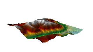
This is a 2-D jpeg image from the 3-D image in ArcScene. I adjusted the image to reflect the elevation. I have added hillshade and adjusted the color ramp to enhance the image. I also rotated the image so that the 3-D aspect can be more easily scene. This is hard to do in 2-D, but I could not find a way to capture the image in 3-D and export it to the blogger without problems.

Week 11 Map 3: Zonal Reclassification

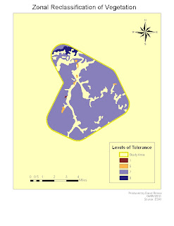
This is deliverable 4 for week 11. The assignment was to reclassify vegetation for study area only. So following instruction from module we used the remap to reclassify the drought tolerance for vegetation in the study area.I chose the color ramp because it is easily distinguishable between levels of tolerance. The no data areas are white. I was able to add all reqquired elements of the map including a legend, neatline, scale bar, north arrow, and source data.

Week 11 Deliverable 3: Model Snapshot

This is the snapshot of my model. The model was run in ArcMAP with modelbuilder.

Week 11 Map 2: Recreation

This is second of 5 deliverable for the week. It showcases the ability to label features using ArcMap 9.3 I followed the instruction in module 1 " add custom text to your maps" to include feature labels of water bodies and recreation features.

Week 11 Map 1: Cities and Roads

This is the first of 5 deliverables for this week. I have followed instructions layed out by Module 1 on Labeling and Annotation. I included all of the required map elements except for a legend which was too excessive.

Week 10: Spring Break Lab

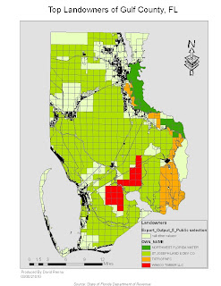
In this lab, We used raw data from tables which were created in ArcMap. We joined the data from the tables to already existing shapefiles.I then exported the data to become a new layer in ArcMAP. The last thing I did was categorize the data with the top 4 landowners of Gulf County, FL. By changing the background color of the layout, you can easily see each parcel and its owner, while leaving the other parcels owned by people or companies not in the top four a neutral color.

Map Overlays and Buffers

Question 1: Which tool did you use? Was there any noticeable difference in its result and the results from the instruction?

I used the Intersect Tool because the description of what the Intersect Tool seem to do is what is being asked of us.This seemed to work much faster and with no noticeable difference in its results. This tool work much quicker than all of the steps taken in the instructions.

Question 2: Which tool did you use here and Why?

I used the Erase tool becaquse we want to keep everything in our original area while getting rid of the aarea within the conservation areas so that the people and the plants are safe from harm.

Question 3: How many features are in this layer? What is the are of the largest feature? What is the are of the smallest feature?

I got 78 features. The largest area was 7765034.5 Square Meters. While the smallest feature was 748.1 Square Meters in area.

Week 8: Image Editing

This is the edited image of the University of West Florida. It is the same image that we worked with last week with a few edits. There is a new shapefile layer named Athletic_fields and Ihave digitized the Athletic Fields into this layer and displayed the layer in my legend. There are also edits to the building layers where the two building have been editied to fit the image. Also I digitized the maintenance road in the lower right portion of the image to the roads layer.

Week6 Georeferencing Repost

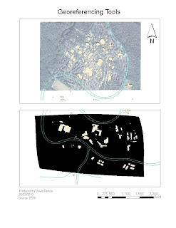
I was able to finally get it to work. I updated my second map. In this map I used 27 points to produce a 3rd linear equation map. It was reported an RMS of 18.58516.
As I mentioned inj my first post. The top map uses 10 critical points and has a 1st order equatioon RMS of 15.89071. I beleive that both maps are of good quality with RMS values under 20 as requested.

Week6: Georeferencing

In this lab, we are georeferencing a unknown aerial to a known buildings and roads map. In order to do this, I added ten control points from the known maps to the georeferenced map or unknown map. After adding the ten points, I displayed data as a table in order to see how similar the two maps were in a 1st ordeer polynomial reference frame. In order to make sure the maps line up we are looking at the RMS or Residual Error. For the map to be a good fit, we are looking for a RMS of under 20. I was able to reduce this number through trial and error to 15.89071 on my maps. This seems to be a very good fit by visualization and the fact my RMS is low.
The second map is a raster map of the same general area.I used a third order polynomial reference frame. I had to use 21 different control points for this map. I got a RMS of 17.83217. A good fit for this size data set.
I don't know why the image is black. When I did the assignment it raster image was fine and matched up well. I even tried to reload the data to my map and it looked like this. I could not remedy the problem. Though you can see by the distortion of the map that it has been Georeferenced.

Week5 Map 2

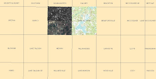
Inb the second map of this assignment. I downloaded and extracted the DRG for Lake Jackson Quad 5335. Then I downloaded and added each of the four quadtants of the South Havana 5336. I found two different version of the information. For the top half I used the Black and White data and on the Southern two I used the color version of the data.
I was not able to convert the DEM for Midway 5236 to the south of South Havana. I did put alot of effort into this assignment and I hope that the time spent is considered.

Week 5 Map 1

This was by far the hardest assignment to date. I had real problems with understanding where to find files that were not corrupt.
This is a map of Gadsden County, Fl. I was able to produce this map with shapefiles downloaded from FGDL website. I then clips the size of each piece of information down to the size of Gadsden County using ArcToolbox.

Haiti Map Post

Week 4 Maps: Projections